Spreadsheet
Basic Concepts
The Spreadsheet is the main part of LabPlot when working with data and consists out of columns. Column is the basic data set in LabPlot used for plotting and data analysis. Every column of the Spreadsheet consists of cells and is specified by its name and the type of the data:
Double - floating-point numbers with double precision for decimal values (range: ±1.79769 × 10308)
Integer - whole numbers, 32-bit signed integers (range: -2,147,483,648 to 2,147,483,647)
Big Integer - large whole numbers, 64-bit signed integers (range: -9,223,372,036,854,775,808 to 9,223,372,036,854,775,807)
Text - alphanumeric strings and text data
Date & Time - date and time values
For each type different representation formats can be assigned like decimal or scientific format for numeric columns etc. In addition to these properties it is also possible to specify the plot designation that is used in some places to to automatically recognize how to plot the data and which columns to use as X, Y, etc.
Data Structure
There are two commonly used ways to structure the data in the spreadsheet - the “wide” format and the “long” (or “tidy”) format. In a wide format, each subject has a single row, and various attributes or time points are spread across multiple columns (e.g., time series data where each time point is a column). For tidy data, each variable is a column and each observation is a row.
For the following example in the wide format for the score obtained by students in three tests
Name |
Test 1 |
Test 2 |
Test 3 |
|---|---|---|---|
Alice |
85 |
90 |
88 |
Bob |
70 |
75 |
80 |
“Test Number” and “Score” are the actual variables, while “Name” is an identifier. In the tidy format, the same data would be structured as follows:
Name |
Test Number |
Score |
|---|---|---|
Alice |
Test 1 |
85 |
Alice |
Test 2 |
90 |
Alice |
Test 3 |
88 |
Bob |
Test 1 |
70 |
Bob |
Test 2 |
75 |
Bob |
Test 3 |
80 |
Important
While both formats are valid and supported in LabPlot, attention needs to be paid to the way how LabPlot operates on the data - namely, for the visualization and analysis, LabPlot always operates on columns and not on rows and therefore different data formats will produce different results.
For example, visualizing the data for both formats in a Bar Plot will produce the following results:
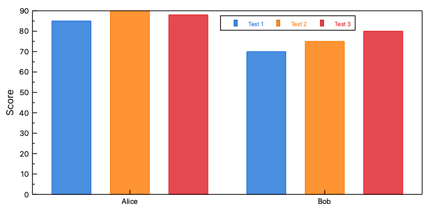
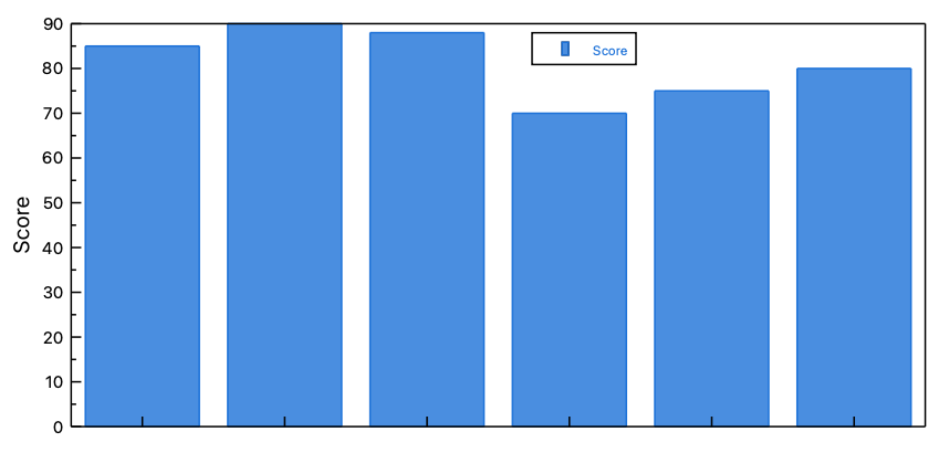
In the first case, the visualization of the three numerical columns with the scores in a bar plot leads to a “grouped” bar plot with three bars - each bar represents a score and each group represents a student name. In the second case, the visualization of the “Score” column (the only numerical column in the spreadhseet) leads to a bar plot with six separate bars - one bar for the score values for each combination of “Name” and “Test Number”.
Import Data
Generate Data
Column Formulas
Columns can be populated with values calculated from formulas. The formula system supports over 600 mathematical, statistical, and scientific functions from the GNU Scientific Library (GSL).
Quick Example:
# Calculate distance from origin
sqrt(x^2 + y^2)

# Normalize data (z-score)
(value - mean(value)) / stdev(value)

# Conditional logic
if(temperature > 0; 1; 0)
To generate values using a formula, select the target column and navigate to the section Formula in the Properties Explorer. Enter your expression, map variables to columns, and enable Auto Update for automatic recalculation on data changes in the source columns and Auto Resize to automatically adjust the size of the target column based on the number of rows in the source columns. The formula system supports referencing other columns in the same spreadsheet or even columns from other spreadsheets within the same project.
For detailed information about syntax, available functions, and examples, see Column Formulas.
Random Values
Columns can be filled with random values from 36 different statistical distributions including Gaussian (normal), uniform, exponential, Poisson, binomial, and many more.
Common distributions:
Gaussian (μ, σ) - Normal distribution for natural phenomena
Uniform (a, b) - Equal probability over a range
Exponential (λ) - Waiting times between events
Poisson (λ) - Count data (number of events)
Binomial (p, n) - Success/failure trials
To generate random values, select one or more columns, right-click and choose Fill with Random Values. Configure the distribution parameters and optionally set a seed for reproducible results.
For a complete guide to all distributions, parameters, and use cases, see Generate Random Values.
Other Generation Methods
In addition to formulas and random values, several utility functions are available in the Generate Data context menu for selected columns:
Row Numbers
Fill columns with sequential row numbers (1, 2, 3, …). The column type is automatically set to Integer.
Usage: Select column(s) → Right-click → Generate Data → Row Numbers
Use cases:
Create index columns
Number observations sequentially
Generate unique identifiers
Const Values
Fill columns with a user-specified constant value. An input dialog prompts for the value based on the column type (numeric, text, etc.).
Usage: Select column(s) → Right-click → Generate Data → Const Values
Use cases:
Initialize columns with default values
Fill baseline or reference values
Set placeholder data
Equidistant Values
Generate arithmetic sequences with precise control over start, end, increment, or count. Three generation modes are available:
Fixed Number - Specify start value, end value, and number of points
Fixed Increment - Specify start value, increment size, and number of points
Fixed Number & Increment - Specify start value, increment, and number (end value calculated)
Usage: Select column(s) → Right-click → Generate Data → Equidistant Values
Examples:
Linear time axis: start=0, end=10, number=100 → [0, 0.101, 0.202, …, 10]
Regular intervals: start=0, increment=0.5, number=20 → [0, 0.5, 1.0, 1.5, …]
Custom sequence: start=5, increment=3, number=10 → [5, 8, 11, 14, …]
Equidistant Date & Time Values
Generate date/time sequences with configurable units (years, months, days, hours, minutes, seconds, milliseconds).
Usage: Select column(s) → Right-click → Generate Data → Equidistant Date & Time Values
Examples:
Daily data: 2024-01-01, increment=1 day, number=365
Hourly logs: 2024-01-01 00:00, increment=1 hour, number=24
Monthly reports: 2024-01-01, increment=1 month, number=12
Sample Values
Downsample or subsample column data using two methods:
Periodic - Take every N-th value (e.g., every 10th point)
Random - Select random subset based on uniform distribution
Usage: Select column(s) → Right-click → Generate Data → Sample Values
Use cases:
Reduce data density for plotting
Extract representative subset
Downsample high-frequency measurements
Note
Sampling creates new columns with the sampled data; original columns remain unchanged.
Flatten Columns
Combine multiple columns into a single column by stacking values vertically. Optionally include reference columns that are repeated for each flattened value (useful for converting wide format to long/tidy format).
Usage: Select columns to flatten → Right-click → Generate Data → Flatten Columns
Example: Converting wide to long format:
# Wide format (2 columns):
Name     Score
Alice    85
Bob      90

# Select Score columns from multiple tests
# Add "Name" as reference column
# Result (long format):
Name     Score
Alice    85
Alice    90
Bob      85
Bob      90
Use cases:
Convert wide format to tidy/long format for analysis
Combine multiple measurement columns
Prepare data for grouped visualization
Manipulate Data
LabPlot provides comprehensive tools for transforming and cleaning column data through the Manipulate Data context menu. All operations support undo/redo and work on multiple columns simultaneously.
Main categories:
Arithmetic Operations - Add, subtract, multiply, divide by values or statistical measures
Add/subtract custom values, mean, median, min, max
Advanced baseline subtraction using arPLS algorithm
Multiply/divide for unit conversions and scaling
Data Filtering - Drop or mask values based on criteria
Drop Values - Permanently remove values (outliers, invalid data)
Mask Values - Temporarily exclude from plots and analysis (preserves original data)
Normalization (15 methods) - Scale data for comparison
Basic: Divide by sum, min, max, count
Central tendency: Divide by mean, median, mode
Spread: Divide by range, SD, MAD, IQR
Standardization: Z-scores (SD, MAD, IQR)
Rescale to arbitrary interval [a, b]
Transformations - Tukey’s Ladder of Powers
x³, x², √x, log(x), 1/√x, 1/x, 1/x² - improve normality, stabilize variance
Data Reordering - Reverse column order
Usage: Select column(s) → Right-click → Manipulate Data → Choose operation
For detailed information about all operations, parameters, and use cases, see Manipulate Data.
Mask Data
Sometimes it is required to ignore some data points in the visualization or when performing some data analysis like fitting etc. To exclude some data points from plotting and data analysis without deleting them, masking of those data points can be used. You can mask the selected data points in the Spreadsheet ( / from the Spreadsheet cell context menu).
In the example below a fit was performed to the original data containing some obvious measurement errors and a fit where those outliers were masked.
Note
Masking can also be done based on value criteria using Manipulate Data → Mask Values. See Manipulate Data for details.
Keyboard Shortcuts
The spreadsheet supports the following keyboard shortcuts for efficient data manipulation:
Editing Operations
Key/Mouse Event |
Function |
|---|---|
Ctrl+C |
Copy selected cells |
Ctrl+V |
Paste into selected cells |
Ctrl+X |
Cut selected cells |
Del or Backspace |
Clear content of selected cells |
Insert |
Insert column (if column selected) or row |
Search and Replace
Key/Mouse Event |
Function |
|---|---|
Ctrl+F |
Open search dialog |
Ctrl+H |
Open search and replace dialog |
Escape |
Close search/replace dialog |
View Operations
Key/Mouse Event |
Function |
|---|---|
Ctrl++ or Ctrl+= |
Zoom in |
Ctrl+- |
Zoom out |
Ctrl+0 |
Reset zoom to 100% |
Ctrl+Mouse Wheel |
Zoom in/out |